library(tidyverse)
library(correlation) # for correlation tests
library(GGally) # for nice correlation plotsSkills Lab 07: Correlation and Chi-square
Setup
Packages and data
Load the necessary packages:
Data
Load the data:
games_tib <- readr::read_csv("data/video_games_data.csv") Variables in the dataset:
- id: Participant’s ID
- age: Participants age
- game: Name of the video game
- game_type: Game classification as “Shooter”, “Sports game”, “RPG” or “Animal crossing”
- affect: Level of emotional affect measured from -6 (most negative) to + 6 (most positive)
- affect_cat: Categorical version of the affect variable, with values “Negative” or “Positive”
- life_sat: life Satisfaction
- experience: Experience of playing video games (0-100)
- hours: Hours spend playing video games per week
Correlation
Task 1: Create a correlation matrix
A good first step in an analysis is to explore the associations between variables
Select the continuous (numeric) variables in the dataset. Save this selection of columns in a new object called
games_tib_corCreate a correlation matrix (either numeric or visual)
The reason we’re selecting numeric variables is because functions cor() and GGally::ggscatmat() will calculate correlations for us, and this can only be done for numeric variables (doubles, integers, etc).
If you encounter an error like this:
Error in cor() : 'x' must be numeric
it means we’re trying perform a calculation on a variable that isn’t numeric. This can happen with the cor() function, but it might pop up essentially with any function that performs mathematical functions (like mean or median).
games_tib_cor <- games_tib |>
  dplyr::select(age, affect, life_sat, experience, hours)
Note how we’ve also saved into a new object called games_tib_cor using the assignment operator, instead of just saving over the same object. By selecting only 5 columns, we’re making a substantial change to the dataset. So it’s good to keep the original version of games_tib available in case we need it later (which in this case, we will do).
games_tib_cor |> cor() age affect life_sat experience hours
age 1.0000000 0.14646774 0.111745366 0.49100762 0.171203480
affect 0.1464677 1.00000000 0.631929165 0.04129028 0.018558241
life_sat 0.1117454 0.63192917 1.000000000 0.03644992 0.005614853
experience 0.4910076 0.04129028 0.036449923 1.00000000 -0.012494233
hours 0.1712035 0.01855824 0.005614853 -0.01249423 1.000000000games_tib_cor |> GGally::ggscatmat()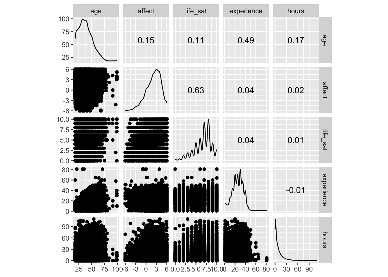
We also talked about how the objects produced by GGally are ggplot extensions, which means that we can modify the plots as we usually would, for example by adding a theme:
games_tib_cor |>
  GGally::ggscatmat() +
  theme_minimal()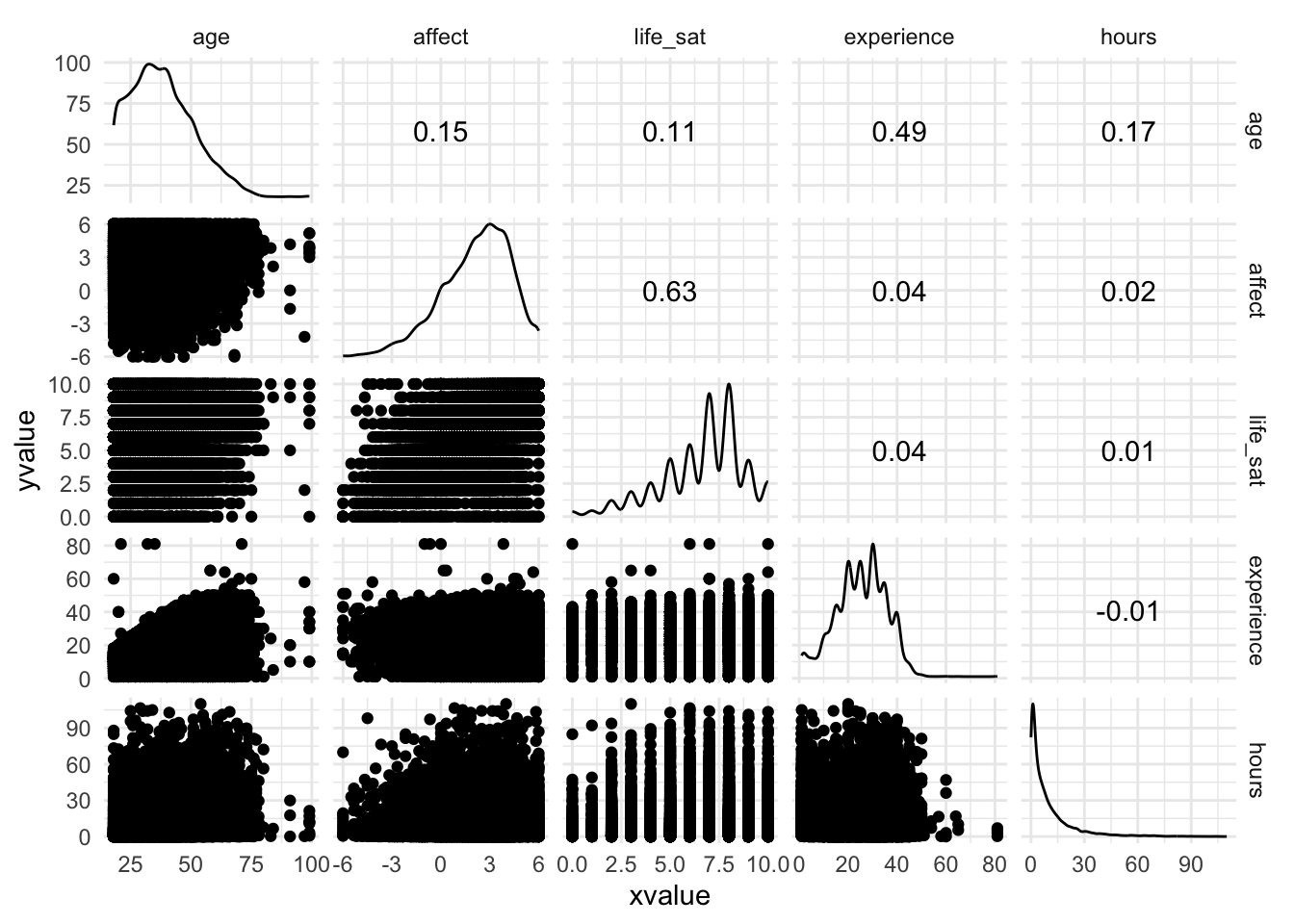
Task 2: Run correlation tests
Run correlation tests on the numeric variables
Which relationships are statistically significant?
The previous functions tell us the sizes of the correlation coefficients but we don’t know whether the relationships are statistically significant. That is, if in reality, the relationship between the variables doesn’t exist, how likely are we to find a correlation coefficient as large as the one we observed in a sample?
correlation::correlation(games_tib_cor)# Correlation Matrix (pearson-method)
Parameter1 | Parameter2 | r | 95% CI | t(16977) | p
-------------------------------------------------------------------------
age | affect | 0.15 | [ 0.13, 0.16] | 19.29 | < .001***
age | life_sat | 0.11 | [ 0.10, 0.13] | 14.65 | < .001***
age | experience | 0.49 | [ 0.48, 0.50] | 73.44 | < .001***
age | hours | 0.17 | [ 0.16, 0.19] | 22.64 | < .001***
affect | life_sat | 0.63 | [ 0.62, 0.64] | 106.24 | < .001***
affect | experience | 0.04 | [ 0.03, 0.06] | 5.38 | < .001***
affect | hours | 0.02 | [ 0.00, 0.03] | 2.42 | 0.047*
life_sat | experience | 0.04 | [ 0.02, 0.05] | 4.75 | < .001***
life_sat | hours | 5.61e-03 | [-0.01, 0.02] | 0.73 | 0.464
experience | hours | -0.01 | [-0.03, 0.00] | -1.63 | 0.207
p-value adjustment method: Holm (1979)
Observations: 16979The column titled r contains the correlation coefficients, while the p-values in the column p. The are some large correlations - like the one between age and gaming experience, or affect and life satisfaction - that are statistically significant. This makes sense.
What makes less sense is that we also have some minuscule correlations that are close to 0, like affect and hours spent playing video games. The correlation is just 0.02, but the p-value is 0.047, which is just statistically significant. Note at the end of the table we have the number of observations listed, which in this case is nearly 17000. At a sample this large, almost everything will be statistically significant. It’s important to always consider effect size (correlation coefficient, mean difference, etc), not just the p-value.
Chi-square
Hypothesis
There will be an association between type of game (Animal Crossing vs Sports Game) and experiences of positive or negative affect.
- Make a prediction! Who do you think is going to be more likely to experience positive affect? Players of Animal Crossing or players of sports games (car racing)?
The main difference here is that we’re now using the the categorical version of affect (positive vs negative) so both variables are categorical.
Task 3: Quick data cleaning
- We’re interested in comparing the game “Animal crossing” against games classified as “Sports game” - filter the rows that only contain these two game types and save the new dataset into an object called
games_tib_chi
Here’s a quick tip on how to check which values are present in a given column if we need to get their exact spelling etc:
games_tib$game_type |> unique()[1] "Animal crossing" "Shooter" "RPG" "Sports game" Filter the right rows and check values again:
games_tib_chi <- games_tib |>
  dplyr::filter(game_type == "Animal crossing" | game_type == "Sports game")

games_tib_chi$game_type |> unique()
[1] "Animal crossing" "Sports game" Note: remember how we didn’t over-write our dataset when working with correlations? It’s good that we didn’t, because now we needed to use it again. If we had over-written it, we’d need to re-read the dataset, mess up the order in which the code naturally progresses, and that’s where 95% of rendering problems typically occur.
Task 4: Plotting!
Create a bar plot (yes, a bar plot!) showing the counts of participants across the two game types split by affect valence
Interpret the plot - does this it support your prediction?
If time left:
Change the default colours
Adjust axis labels
This is what we did in the session:
games_tib_chi |>
  ggplot2::ggplot(aes(x = game_type, fill = affect_cat)) +
  geom_bar(position = "dodge")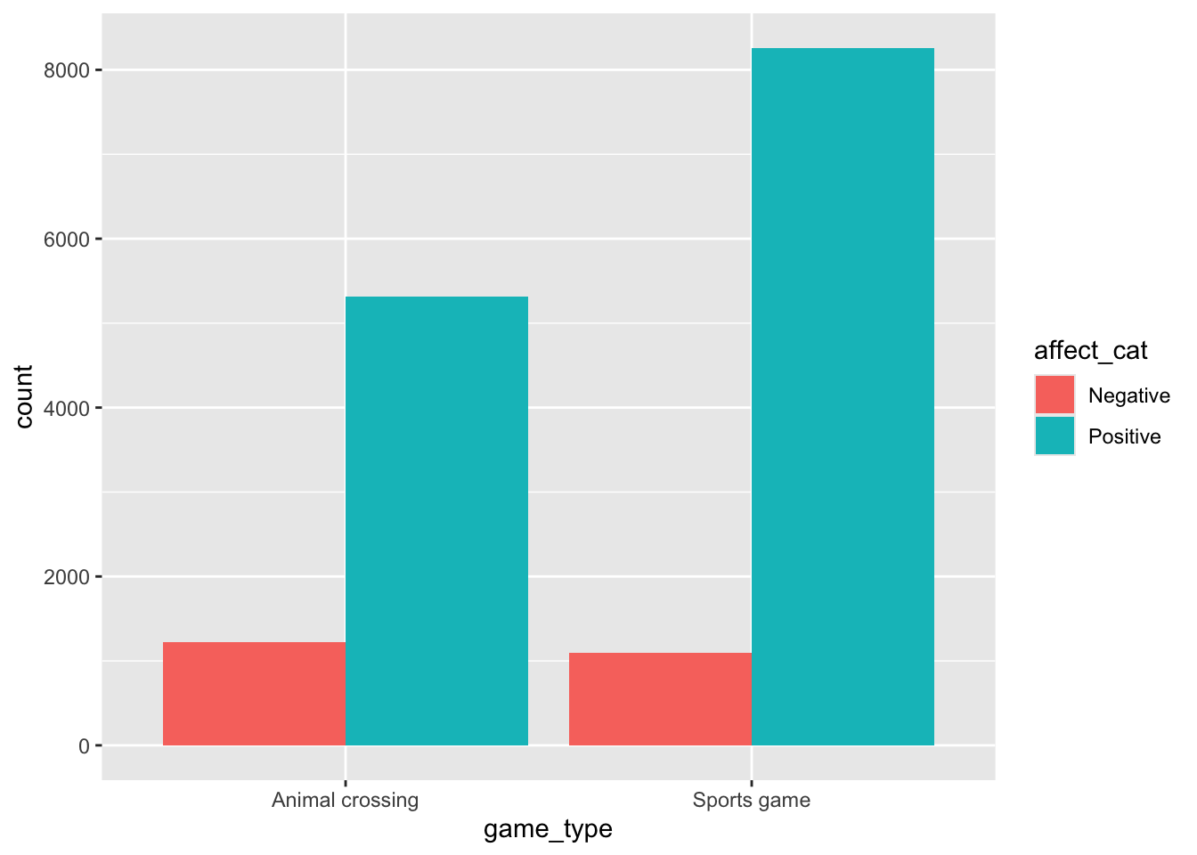
The tutorial has a detailed breakdown of making plots like this so make sure to check it out. I just want to highlight that yes, we’re making a bar graph, but it’s a bar graph with counts - for all intents and purposes, this is the same use as a histogram, which is why I don’t consider it to be as big of a crime.
Some additional code to make the plot prettier:
games_tib_chi |>
  ggplot2::ggplot(aes(x = game_type, fill = affect_cat)) +
  geom_bar(position = "dodge", width = 0.75) +
  scale_fill_manual(values = c("darkmagenta", "darkcyan")) +
  labs(x = "Type of game", y = "Count", fill = "Affect category") +
  theme_light()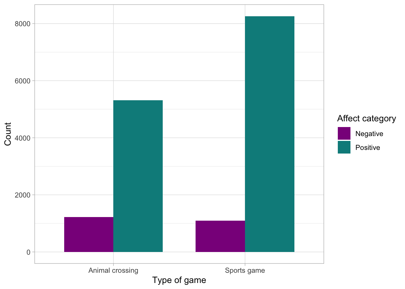
Finally, I briefly showed how to to convert each group into equal proportions to make comparisons easier. In the code below, I’m replacing position = "dodge" with position = "fill" . This will make the proportions comparable, even if our sample sizes aren’t equal:
games_tib_chi |>
  ggplot2::ggplot(aes(x = game_type, fill = affect_cat)) +
  geom_bar(position = "fill", width = 0.75) +
  scale_fill_manual(values = c("darkmagenta", "darkcyan")) +
  labs(x = "Type of game", y = "Count", fill = "Affect category") +
  theme_light()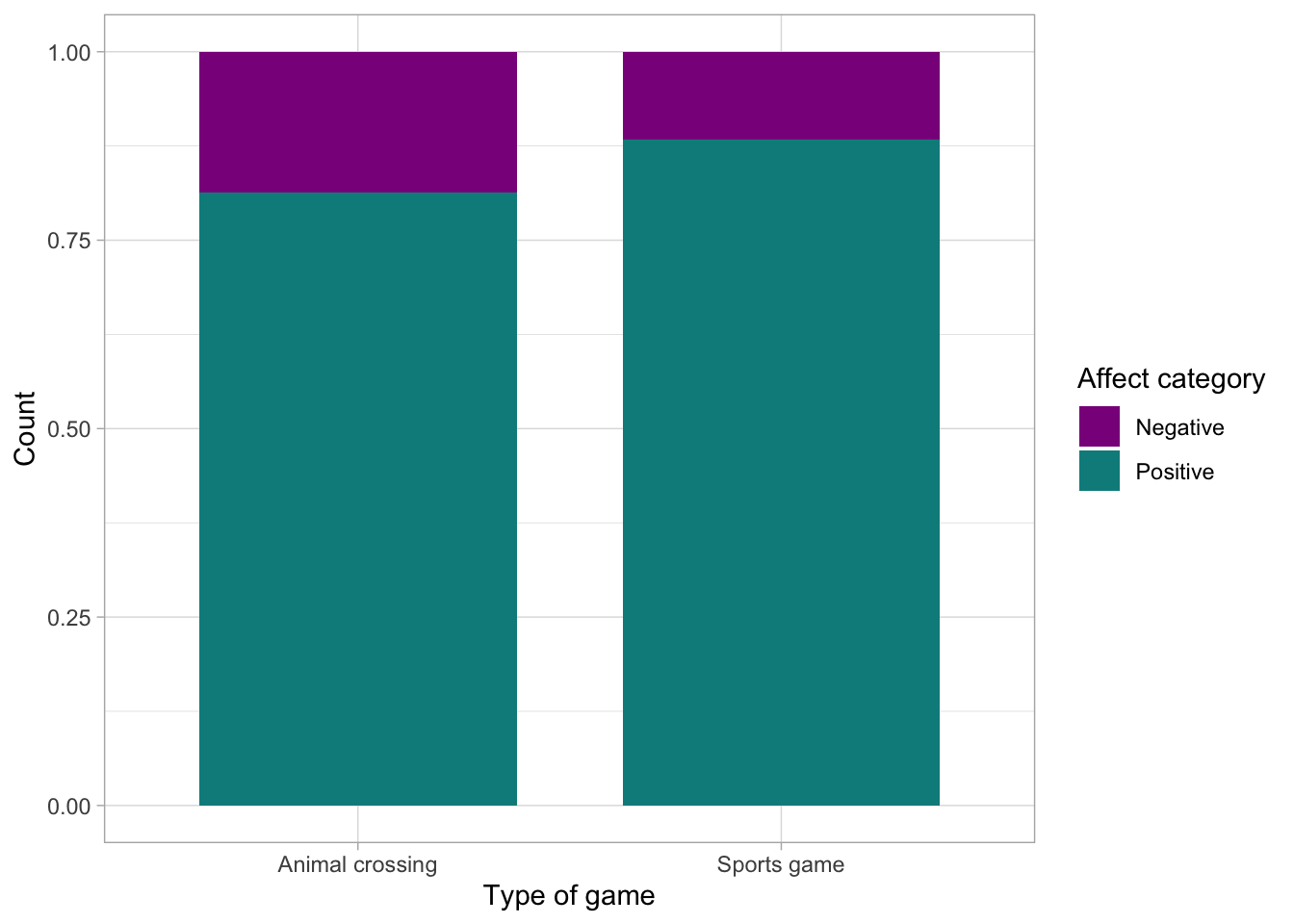
Task 5: Run Chi-square test
Run the test of association between type of game and affect category
Interpret the results - does the statistical test support your prediction?
Can we reject the null hypothesis?
Can we say that a specific type of video game causes a type of affect?
chi_test <- chisq.test(games_tib_chi$game_type, games_tib_chi$affect_cat)
chi_test
    Pearson's Chi-squared test with Yates' continuity correction

data:  games_tib_chi$game_type and games_tib_chi$affect_cat
X-squared = 147.94, df = 1, p-value < 2.2e-16
The chi-square test compares the two things: the counts/frequencies we would expect in every combination of the category if the null is true. That is, if the two variables are not associated whatsoever. These expected frequencies are then compared against the frequencies we actually observed in the dataset. We can ask R to print out both:
chi_test$expected games_tib_chi$affect_cat
games_tib_chi$game_type Negative Positive
Animal crossing 950.5018 5580.498
Sports game 1361.4982 7993.502Take the row for “Animal crossing”. If there is no association between the categories, we would expect to see 950.5018 individuals experiencing negative affect and 5580.498 individuals experiencing positive affect. We can take their ratio:
5580.498 / 950.5018[1] 5.871107This tells us that those who play Animal crossing are 5.87 more likely to experience positive affect. How about Sports game players?
7993.502 / 1361.4982[1] 5.871107Same ratio. These are our expectations under the null hypothesis - i.e. under the null, we expect these ratios to be the same. What we do next is that we look what we actually observed in the data:
chi_test$observed games_tib_chi$affect_cat
games_tib_chi$game_type Negative Positive
Animal crossing 1217 5314
Sports game 1095 8260For animal crossing the ratio is:
5314 / 1217 [1] 4.366475so the players are only 4.37 times more likely to experience positive affect. For sports games players:
8260 / 1095[1] 7.543379The ratio is much higher. This aligns with the statistically significant effect we detected with the chi-square test.
References:
Video games and well-being paper source of the dataset):