library(tidyverse)
library(ggdogs)Skills Lab 08: The linear model (1)
Live google doc: linktr.ee/analysingdata
Today’s Session
Visualising linear models
Fitting a linear model with one predictor
Interpreting model coefficients
Using our model to make predictions
Kahoot!
The Data
Researchers wanted to see whether pet dogs will rescue their owners in a variety of scenarios. They collected information about each dog, including their size, age, sex, and then measured how long it took the dog to rescue their owner who was trapped in a box.
Full file path:
Cloud/project/data/dog_rescue.csvRelative file path:
data/dog_rescue.csv
Research question:
Can we use dog size to predict the time it takes the dog to rescue their trapped owner?
Hypotheses:
We’re not testing a hypothesis in this session (not with p-values anyway). We’re going to use R to figure out what kind of line best summarises our data. We’ll test some hypotheses next week.
We can still make an informal prediction though.
What kind of relationship do you think there is between dog size and the time it takes a dog to rescue their human? In other words, who do you think is going to be faster to rescue their human - smaller dogs or larger dogs?
Read in the Data
dog_tib <- readr::read_csv("data/dog_rescue.csv") dog_name- name/id of the dogsex- dog’s sex; coded as 1 for “yes”, 0 for “no”. That’s all the info the authors have provided ¯\_(ツ)_/¯rescue_time_sec- time (in seconds) it took the dog to rescue their trapped ownervocal_distress_owner- rating of how distressed the owner sounded when calling for help, on a scale 1 (not very distressed) to 6 (very distressed)age_months- age of the dog in monthsheight_m- height of the dog in metresweight_kg- weight of the dog in kilograms
Task 1: Preparing for the analysis
Make a prediction: who do you think is going to be faster to rescue their human - smaller dogs or larger dogs?
Convert the height variable from metres to centimetres to make it easier to interpret (for your own practice, you can also try converting into inches)
dog_tib <- dog_tib |>
  dplyr::mutate(
    height_cm = height_m*100
  )
Task 2: Plotting
Create a plot showing the relationship between dog height and rescue time.
Include the line of best fit
Interpret the plot:
Is the relationship positive or negative?
What do you think is the value of
What do you think is the value of
Here’s an example of how to complete the plotting task. Specifying the “colour” argument is not crucial but it can be nice if we’re working with a small sample like this: we can see which dot belongs to which dog.
dog_tib |>
  ggplot(aes(x = height_cm, y = rescue_time_sec, colour = dog_name)) +
  geom_point(size = 3) +
  stat_smooth(method = "lm", colour = "darkcyan") +
  labs(x = "Dog height (cm)", y = "Rescue time (sec)") +
  theme_bw()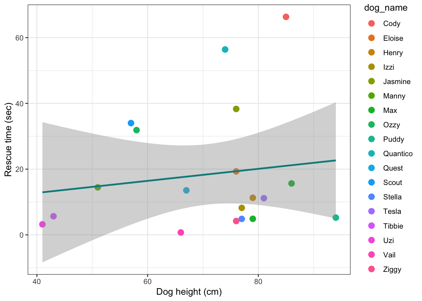
Let’s see if we can give this plot a little more style:
dog_tib |>
  ggplot(aes(x = height_cm, y = rescue_time_sec)) +
  ggdogs::geom_dog(dog = "doge_strong", size = 3) +
  stat_smooth(method = "lm", colour = "darkcyan", fill = "darkblue") +
  theme_bw()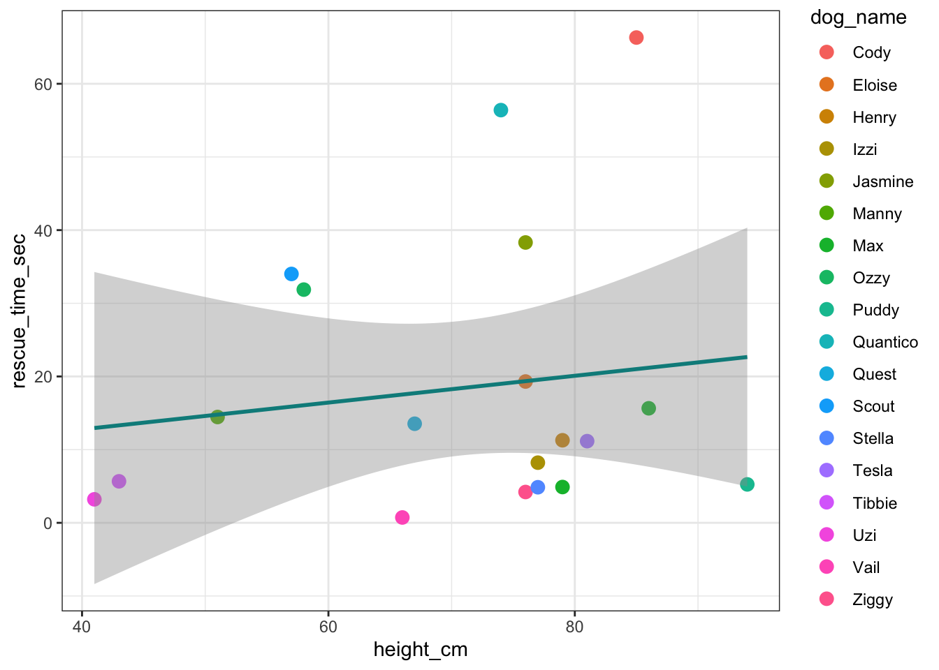
This is just an example of how we can have some fun with ggplot. We probably wouldn’t include a plot like this in a formal report (although… who’s going to stop us?). If you’d like to learn more about the ggdogs package, you can have a look at their github page: https://github.com/R-CoderDotCom/ggdogs and of course, the author also created an equivalent package for cats: https://github.com/R-CoderDotCom/ggcats.
Interpreting plots:
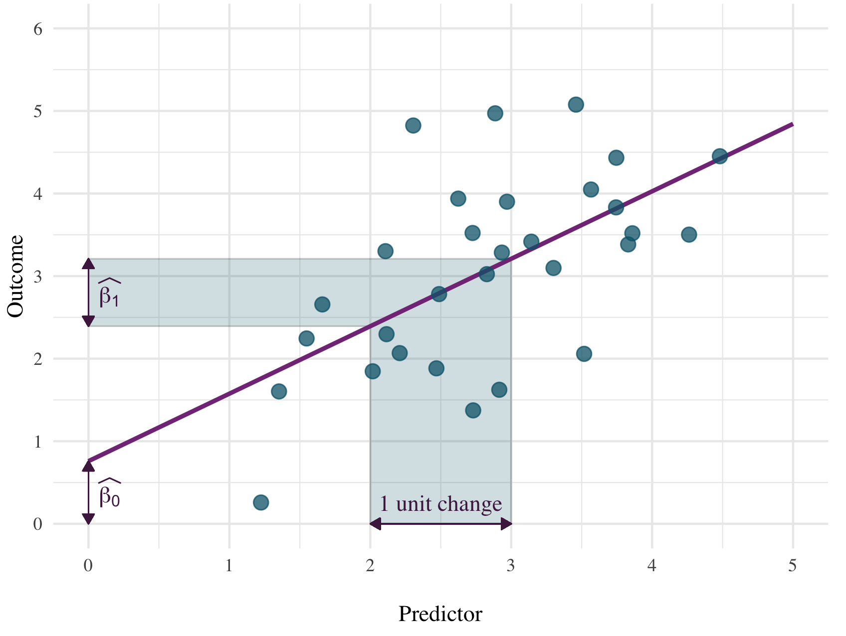
If we want to draw a line through a scatter plot, we need to know two things - one is the intercept. If we were to draw a vertical line going up from the value of 0 on the x axis, the intercept is the the point where our line crosses this 0-line. The intercept is labelled as
The second thing is the slope - i.e. how steep the line is. Because we’re working with linear models, we can take any section of the line and slope will always be the same. When figuring out the slope, we’re asking the question: If we move by 1 unit on the axis, how much higher will the line climb (or what will be the change on the y axis)?
Take a look at the figure below again. Let’s say that we’re increasing from 2 to 3 on the x axis. The line is higher at 3 than it is at 2. What’s the difference in this height? It’s the value labelled as
How about our dog rescue plot? Let’s take a look again. By default, the x axis was cut-off at 40 so I added a line of code that forces the coordinates to start at 0 (+ coord_cartesian(xlim = c(0, 100))). If we extend the line all the way to the left until it crosses the 0-line, we find out intercept. By the looks of it, it could be around the value 5.
dog_tib |>
  ggplot(aes(x = height_cm, y = rescue_time_sec)) +
  geom_point(size = 3) +
  stat_smooth(method = "lm", colour = "darkcyan", fullrange = TRUE) +
  coord_cartesian(xlim = c(0, 100)) +
  theme_bw()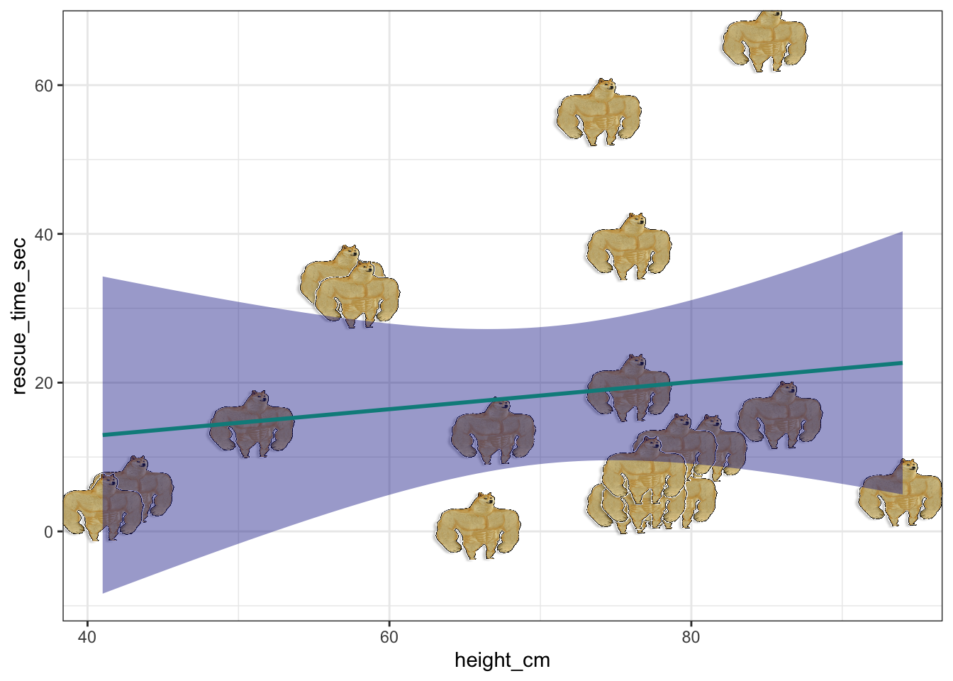
The slope is trickier to guess just from a graph. But let’s do it for the sake of the exercise. I’ve tweaked the coord_cartesian() function again. This time, we’re zooming on the portion of the graph that goes from 75 to 76 on the x axis (because we want an increase one unit) and from 19 to 20 on the y axis (because we want enough zoom to be able to judge the change in the height of the line).
You can see straight away that the line is not very steep. When dog height (x) is 75, the rescue time (y) is about 19.17. When dog height is 76, rescue time is at 19.3. The slope is then 19.3 - 19.17 = 0.13.
dog_tib |>
  ggplot(aes(x = height_cm, y = rescue_time_sec)) +
  geom_point(size = 3) +
  stat_smooth(method = "lm", colour = "darkcyan", fullrange = TRUE) +
  coord_cartesian(xlim = c(75, 76), ylim = c(19, 20)) +
  theme_bw()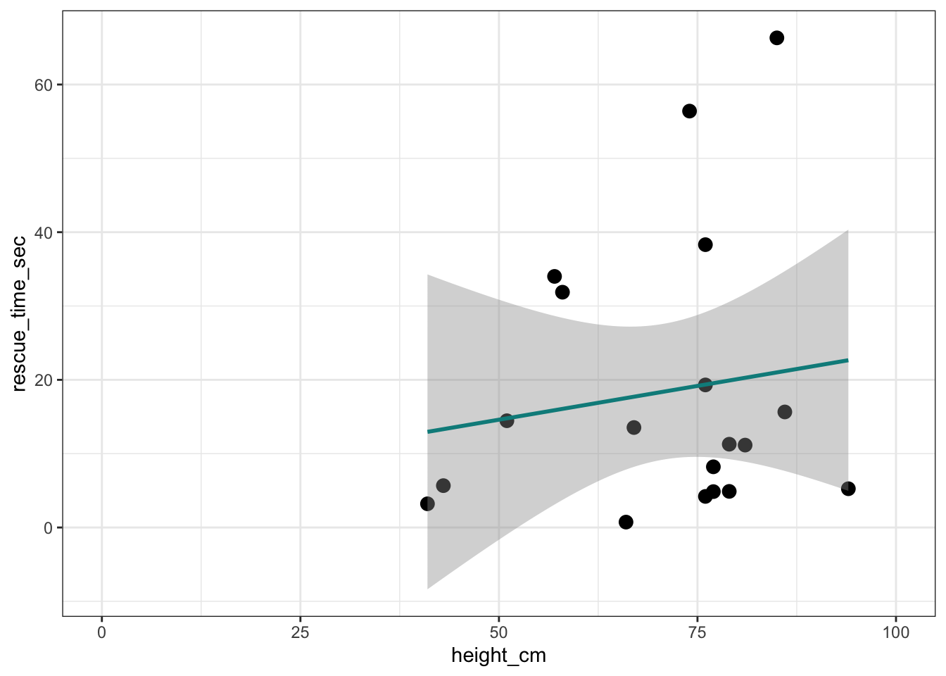
Finally, what’s the “ribbon” around the line? That’s the confidence interval. Note how it’s narrower in the middle. That’s were most of the scores are, so there’s less uncertainty about what the model predicts. It gets wider as we get towards the tails of the dataset.
Luckily, we don’t have to rely on estimates from the plots! We can use R functions to figure out the exact values of the intercept and the slope.
Task 3: Fitting the model
The general equation for the linear model is:
What is the equation for our model?
- Generic form: RescueTime = b0 + b1 (HeightCM)
What is the value of
b0 is the Intercept: 5.45
- Interpreting the intercept
Intercept is the predicted value of the outcome when all other predictors in the model are 0. In our case, it’s the value of rescue time when height is 0. So for a dog of height 0cm (!) the model predicts rescue time of 5.45 seconds. Let’s take a moment to process the absurdity here. The model doesn’t care whether what it predicts is realistic - it just crunches numbers. It’s up to us to decide whether predictions make sense. The model is basically telling us that a microdog with a height of 0cm would rescue us in just over 5 seconds. Unfortunately, the world is not populated by microdogs.
What is the value of
b1 is the Intercept: 0.18
- Interpreting the slope
The slope represents the increase in an outcome associated with an increase of 1 unit in the predictor. In this case, as dog height increases by 1 cm, the model predicts an increase in rescue time by 0.18 seconds. How can we contextualise this? Because this increase is linear (i.e. the steepness of the line doesn’t change), we can do some simple maths. 1 cm is not a lot to differentiate between dogs. How about 10cm? With an increase in height of 10cm, we would expect an increase in rescue time 0.18*10 = 1.8 seconds. Probably still not a huge difference, but these values are easier to interpret. We can also do it the other way around - what kind of difference in height would we need if we wanted to see a change in rescue time of 10 whole seconds? We can work it out by dividing 10 by 0.18: 10 / 0.18 = 55.56. Therefore the model predicts that a dog would have to be 55.56 cm taller to take 10 additional seconds to rescue their human.
Complete the equation with values from the model
- Replace values of b0 and b1 in the equation
- RescueTime = 5.45 + 0.18(HeightCM)
Interpret the results
dog_tib |>
  lm(rescue_time_sec ~ height_cm, data = _)
Call:
lm(formula = rescue_time_sec ~ height_cm, data = dog_tib)

Coefficients:
(Intercept)    height_cm
      5.449        0.183
Task 4: Predicting unknown values
Let’s say that we have a dog who is 36 cm tall. What does our model predict about how long it would take this dog to rescue their human?
Let's have a look at our equation again:
- RescueTime = b0 + b1 (HeightCM)
We now know the values of b0 and b1 , so we can add them into the equation:
- RescueTime = 5.45 + 0.18 (HeightCM)
And then let R do the work:
x <- 36

5.45 + (0.18 * x)
[1] 11.93